AWS Glue Iceberg tables schema can't be updated with Pulumi

In previous blog, we have built a tensorflow model to classify sentiments of movie reviews base on tensorflow and keras high level API, and compile it. In this blog, we will train the model on the movie review dataset to improve the accuracy of the model.

Train Model

To train the model, we need to pass the training datasetand validation dataset into the model. Thetraining datasetis used to train the model and thevalidation dataset` is used to evaluate the model’s performance. Beside, we also need to specify the number of epochs to train the model.

# train the model
history = model.fit(
    train_ds, # training dataset  
    validation_data=val_ds, # validation dataset
    epochs=config.epochs # number of training rounds over the entire dataset
  )

In above code, we are using fit() method to train the model. The fit() method takes two arguments, train_ds and val_ds. train_ds is the training dataset and val_ds is the validation dataset. The epochs argument specifies the number of training rounds over the entire dataset. The fit() method returns a history object which contains the training and validation metrics.

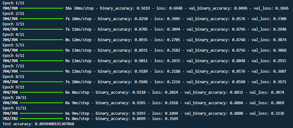
Below is the model training epochos, we defined the epochs as 11, so you can see the there is 11 steps to train the model. Each step is an epoch and displaying the training and validation loss and accuracy.

# the trainning times
epochs = 11

Model Train Epochs

Plot Training Metrics

Base on history object, we can plot the training and validation metrics. We using matplotlib library to plot the metrics.

import matplotlib.pyplot as plt


def display_training_loss_history(trained_history):
    history_dict = trained_history.history
    history_dict.keys()
    loss = history_dict['loss']
    val_loss = history_dict['val_loss']
    epochs = range(1, len(history_dict['binary_accuracy']) + 1)

    plt.plot(epochs, loss, 'bo', label='Training Loss') # "bo" is for "blue dot"
    plt.plot(epochs, val_loss, 'b', label='Validation Loss') # b is for "solid blue line"
    plt.title('Training and Validation Loss')
    plt.xlabel('Epochs')
    plt.ylabel('Loss')
    plt.legend()
    plt.show()


def display_training_accuracy_history(trained_history):
    history_dict = trained_history.history
    history_dict.keys()
    acc = history_dict['binary_accuracy']
    val_acc = history_dict['val_binary_accuracy']
    epochs = range(1, len(acc) + 1)
    plt.plot(epochs, acc, 'bo', label='Training Accuracy')
    plt.plot(epochs, val_acc, 'b', label='Validation Accuracy')
    plt.title('Training and Validation Accuracy')
    plt.xlabel('Epochs')
    plt.ylabel('Accuracy')
    plt.legend(loc='lower right')
    plt.show()

Above code defines two functions to plot the training and validation loss and accuracy. We can call these functions after training the model to plot the metrics. Below is plot graphically of the training and validation loss and accuracy.

Training and Validation Accuracy

Training and Validation Accuracy

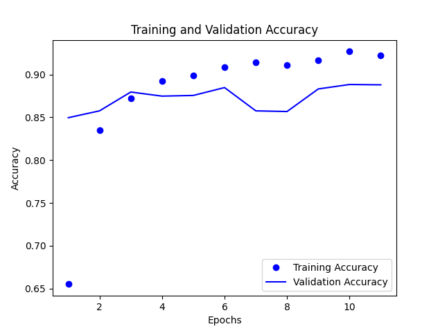
In the above graph, we can see that the training accuracy and validation accuracy are close to each other, which means the model is not overfitting. The training and validation accuracy are increasing.

Training and Validation Loss

Training and Validation Loss

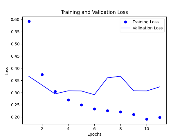
In above graph, we can see that the training loss and validation loss are decreasing. This means the model is improving its performance on the training dataset.

Conclusion

In this blog, we have trained the model on the movie review dataset to improve the accuracy of the model. We have also plotted the training and validation metrics to check the performance of the model. In the next blog, we will evaluate the model on the test dataset.